
Horses near Bozeman, Montana, with the Bridger Range in the distance. Photo courtesy of Scott Bischke.
Key Messages
- Climate models cannot capture the observed global temperature trend from 1880 to present without accounting for natural and human-emitted atmospheric greenhouse gases in the simulations. [high confidence, robust evidence]
- For a given future greenhouse gas scenario, global climate models run by international modeling centers collectively produce similar 21st-century temperature trends with a range or spread in the magnitude of change.
Introduction
In the following chapters we present key aspects of projected 21st-century climate and hydrologic change in the GYA. In this chapter we provide a summary overview of the IPCC climate scenarios and climate models as a basis for understanding what underlies the GYA projections. We also present details of the climate data we use in the Assessment.
Climate Scenarios
Climate scenarios or projections describe plausible pathways for future climate change and provide goals for potentially mitigating such change. There are two, interconnected parts to building climate scenarios. First, assumptions about societal choices, population growth, energy use, existing and future technology, and land-use change are used to establish a range of time-dependent trajectories of future emissions of greenhouse gases (GHGs)—e.g., carbon dioxide (CO2), methane (CH4), nitrous oxide (N2O), and fluorinated gases (e.g., HFCs)—and aerosols (fine particles) into the atmosphere[1] (Moss et al. 2010; Taylor et al. 2012). The emissions trajectories are incorporated into climate models to simulate a range of future climates, typically to the year 2100 and beyond. (See Hayhoe et al. 2017 for further details about scenarios.)
Climate scenarios are re-evaluated with each successive IPCC Assessment Report to include new information as it becomes available. Successive generations of climate models used in the assessments are evaluated for their ability to simulate known past and present changes in climate. Projections of future climate from the models are rigorously analyzed by the scientific community, and the output from the models is used to assess the climate impacts on marine and terrestrial ecosystems, water resources, economies, and human health.
The climate scenarios developed for IPCC AR5 are called Representative Concentration Pathways (RCPs), which is a reference to how much the balance of incoming and outgoing energy in the Earth system is affected by the accumulation of GHGs and aerosols in the atmosphere (Figure 2 7). … RCP8.5 is an upper bound pathway that represents little or no mitigation in the coming decades and results in global warming of about 9°F (5°C) by the end of century. RCP4.5 is an intermediate pathway that results in about 4.5°F (2.5°C) warming. RCP4.5 and RCP8.5 are currently the most widely considered scenarios in climate change research.
The climate scenarios developed for IPCC AR5 are called Representative Concentration Pathways (RCPs), which is a reference to how much the balance of incoming and outgoing energy in the Earth system is affected by the accumulation of GHGs and aerosols in the atmosphere (Figure 2 7). The RCPs bracket a range of plausible atmospheric GHG concentrations in the future based on various levels of emission reductions (mitigation), without assigning likelihood to any pathway.
The number of an RCP indicates the amount of radiative forcing (in watts per square meter, or W/m2) at the year 2100 relative to the baseline year 1750. Radiative forcing is the difference between the energy gained from the sun and the energy radiated back to space. A positive difference means the atmosphere is warming so the higher the RCP value, the greater the potential warming. Four RCPs are considered in AR5 (Figure 4-1): RCP2.6, RCP4.5, RCP6.0, and RCP8.5. In RCP2.6, GHGs peak at mid century and decline thereafter as an outcome of aggressive mitigation, ultimately leading to global warming of about 2.7°F (1.5°C) at end of century as compared to the pre-industrial period (1850-1900). RCP8.5 is an upper bound pathway that represents little or no mitigation in the coming decades and results in global warming of about 9°F (5°C) by the end of century. RCP4.5 is an intermediate pathway that results in about 4.5°F (2.5°C) warming. RCP4.5 and RCP8.5 are currently the most widely considered scenarios in climate change research. Note that these projected temperature changes are global averages over land and oceans and, as evidenced by the continued rate of warming observed in the Arctic today versus other places, the degree of regional warming will vary across the globe.
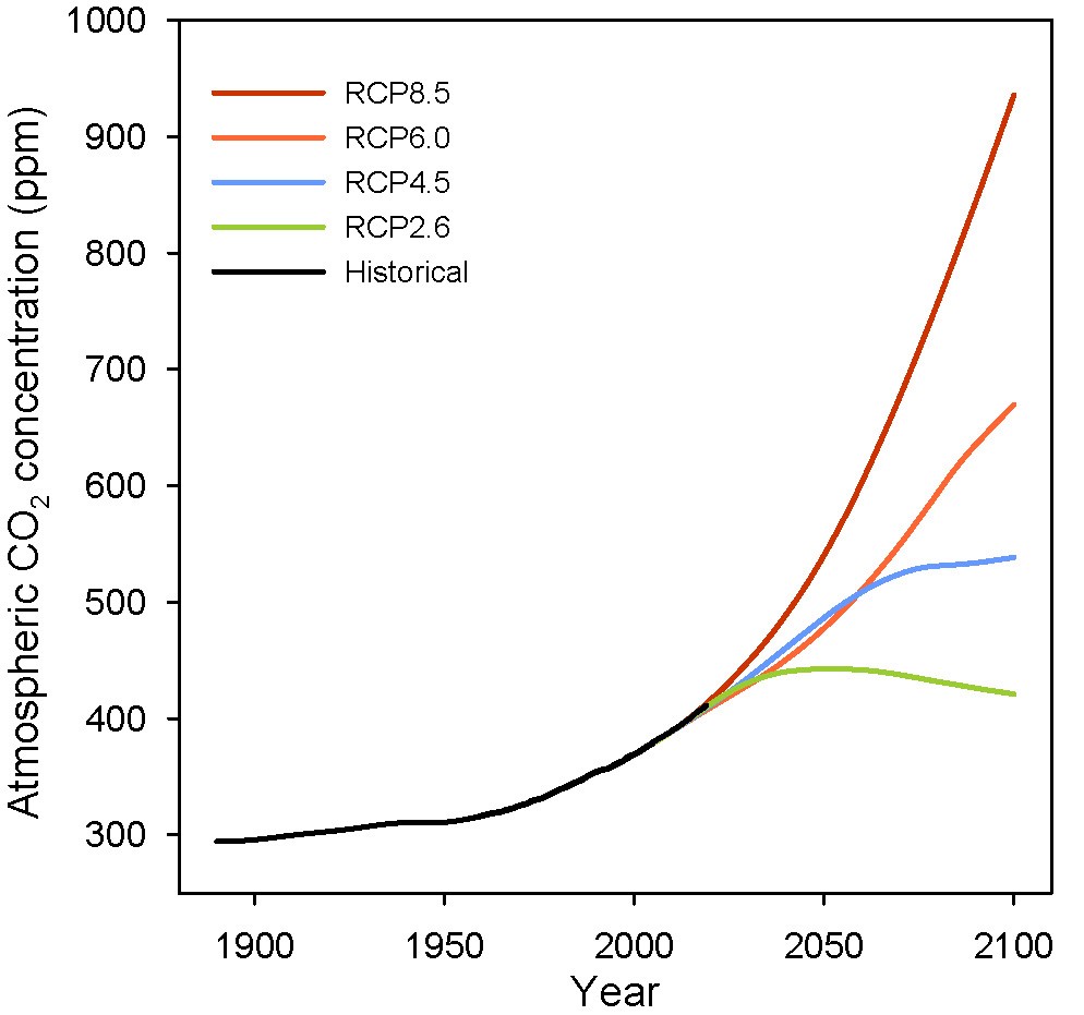
Figure 4-1. Annual average atmospheric CO2 concentrations. The black line combines reconstructed values from 1880-1958 and Mauna Loa observations from 1959-2019. The colored lines are the four Representative Concentration Pathway (RCP) scenarios used in the Fifth IPCC Assessment Report. Mauna Loa observations retrieved from Scripps Institute (undated). RCP2.6 data from van Vuuren et al. (2007); RCP4.5 data from Smith and Wigley (2006), Clarke et al. (2007), and Wise et al. (2009); RCP6.0 data from Fujino et al. (2006) and Hijioka et al. (2008); RCP8.5 data from Riahi et al. (2007). These data sources are compiled at RCP Database (undated).
Climate Models
The geologic, historical, and observational records discussed in Chapters 2 and 3 provide a picture of past and ongoing climate change in the GYA. To explore the complexities of future climate—as well those of the past and present—the international scientific community relies on climate models.
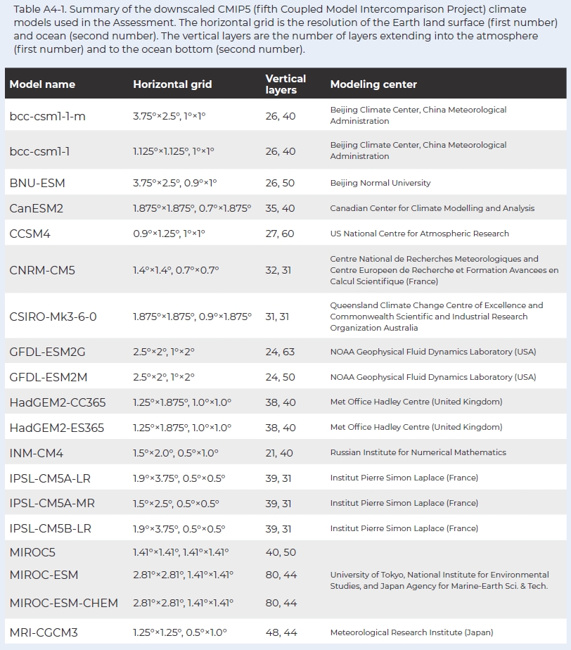
Climate models are numerical models based on the long-known physics that govern the circulation of the atmosphere and oceans. Global climate models (GCMs)[2] used in climate assessments such as the IPCC were originally derived from weather prediction models and have progressively become more complex and comprehensive to be capable of simulating the Earth system. As illustrated in Figure 4-2, GCMs now account for many interrelated processes across time and space (e.g., cloud formation, ocean circulation and heat transport, carbon cycling, soil water, transpiration from a leaf) in response to external and internal drivers (e.g., changes in Earth-Sun geometry, atmospheric composition, solar variability, volcanic eruptions) and internal conditions (e.g., the extent of continental ice sheets, position of the continents, sea level). The models are composed of tens to hundreds of thousands of lines of computer code run on super computers. The 20 models used in this Assessment are described in Table A4-1 of the appendix to this chapter.
[Global climate models] account for many interrelated processes across time and space (e.g., cloud formation, ocean circulation and heat transport, carbon cycling, soil water, transpiration from a leaf) in response to external and internal drivers (e.g., changes in Earth-Sun geometry, atmospheric composition, solar variability, volcanic eruptions) and internal conditions (e.g., the extent of continental ice sheets, position of the continents, sea level). The models are composed of tens to hundreds of thousands of lines of computer code run on super computers.
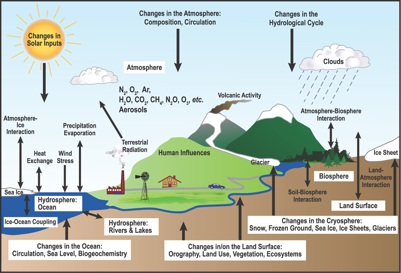
Figure 4-2. Processes and features of the Earth system represented in state-of-the-art climate models. Source: Le Treut et al. (2007).
Global climate models portray the Earth’s climate on three-dimensional grids that are used for numerical computations (Figure 4-3). The horizontal grid boxes in the models in AR5, for example, typically are on the order of 2° in latitude and longitude (about 140 miles by 100 miles [225 km by 160 km] at the latitude of the GYA). The models also include many tens of vertical levels that extend from ocean bottom through the stratosphere (Table A4-1). The models are run on time steps of minutes and output from the simulations (e.g., temperature, precipitation, wind) is recorded at some hourly interval, typically 6 hours, and aggregated into daily and monthly values. The raw output can require petabytes of storage space (a petabyte of storage is roughly equivalent to the capacity of 1000 large home computers).
Spatial resolution for each successive generation of GCMs generally increases (Figure 4-3). Finer resolution models—that take advantage of increased computer capacity and speed—lead to model improvements that better represent atmospheric, oceanic, and surface physics. Extensive details on climate models and climate modeling are given by the National Research Council (2012) and the National Center for Atmospheric Research (NCAR-UCAR undated). The details of the fifth Coupled Model Intercomparison Project (CMIP5) GCMs and their configurations are presented by Flato et al. (2013) as part of the full Fifth IPCC Assessment Report (IPCC 2014).
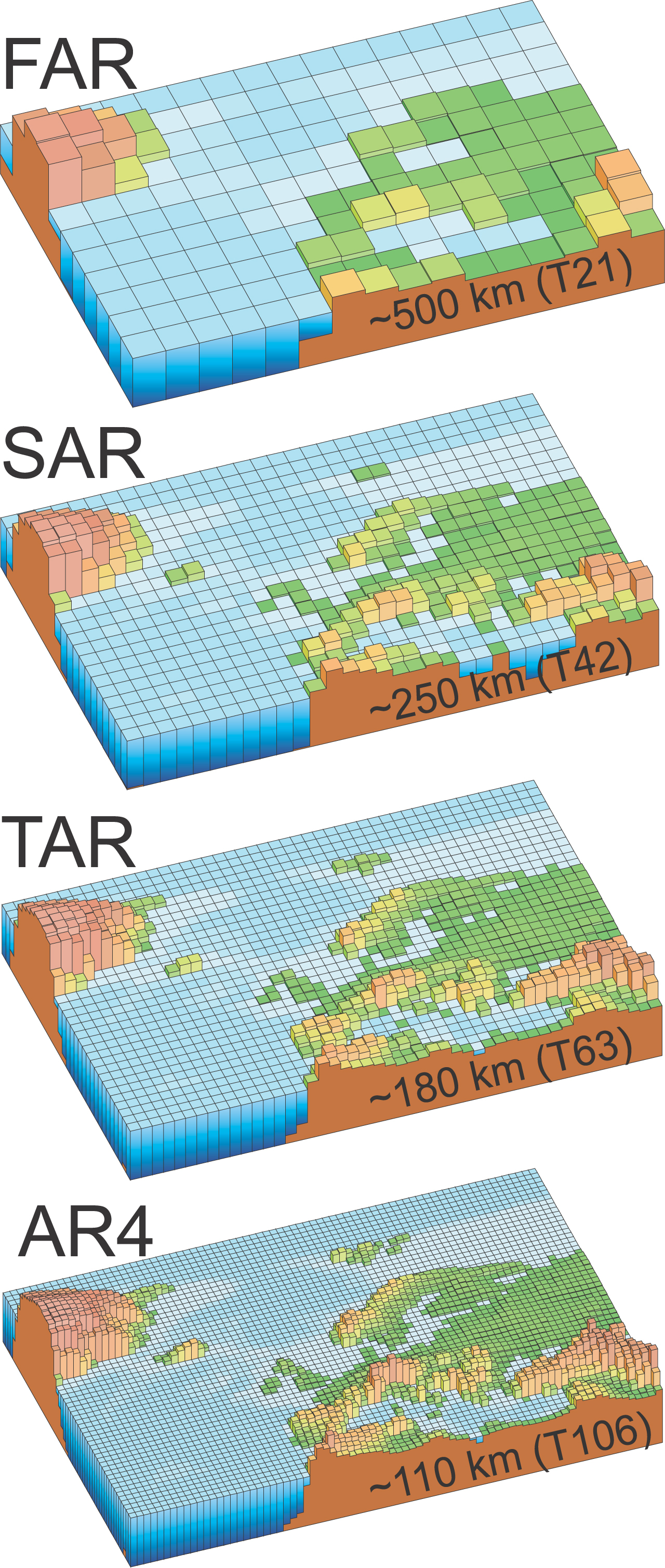
Figure 4-3. Resolution of topography and ocean bathymetry as represent by progressive generations of global climate models used in IPCC Assessment Reports from 1990-2007. The model grid boxes range from about 500 km by 500 km (310 mile by 310 mile) in 1990 to about 110 by 110 km (62 mile by 62 mile) in 2007. FAR: First Assessment Report (1990); SAR: Second Assessment Report (1995); TAR: Third Assessment Report (2001); and AR4: Assessment Report 4 (2007). (Source: Le Treut et al. [2007])
The utility of climate models in GHG-based climate projections and the role of atmospheric GHG concentrations in global warming are clearly demonstrated by comparing long-term modeled global temperature changes with observations (Figure 4-4).

Figure 4-4. Panel (a) Global mean annual air temperature change since 1880 relative to the 1901-1960 mean. In (a) the solid orange line is the average of all CMIP5 (fifth Coupled Model Intercomparison Project) global climate models, the orange shading is the standard deviation of the models, and the dashed orange lines indicate the maximum and minimum range of the models. Three independent estimates of the observed temperature changes are shown by the teal, red, and black lines. The modeled temperature change in panel (a) includes both anthropogenic drivers (e.g., greenhouse gases, land-use change) and natural climate drivers (e.g., solar variability, volcanic eruptions). Note that the models collectively simulate the observed global cooling caused by the eruption of Mount Pinatubo in 1991 (dashed dark orange vertical line). Panel (b) shows the global mean temperature change simulated by climate models (solid blue line, shading, and dashed lines as in [a]) that included the natural drivers but not the anthropogenic drivers. After about 1960, the observed temperature changes diverge substantially from the temperature changes without anthropogenic drivers (see Chapter 3). Thus, both natural and anthropogenic greenhouse gases must be included in the simulations for the models to reproduce the observed warming since 1960, indicating that the warming is to a large part attributable to anthropogenic factors. (Source: modified after Knutson et al. [2017])
[N]atural and anthropogenic greenhouse gases must be included in the simulations for the models to reproduce the observed warming since 1960, indicating that that the warming is to a large part attributable to anthropogenic factors.
Climate models published since the 1970s have been shown to simulate accurately the global warming attributed to atmospheric CO2 in the intervening 50 yr to present day (Hausfather et al. 2020). Similarly, when looking back further, models can only reproduce paleoclimates if they include the appropriate level of GHGs in the simulations. For example, accurate representation of the climate during the Last Glacial Maximum (21,000 yr ago) is only possible when using GHG concentrations from that time, which, based on reconstructions from ice cores, were less than half those of present day. Successful comparisons of model results with paleoclimate and historical data described in Chapters 2 and 3 increases our confidence in the ability of the models to project how the climate system would respond to a given scenario of future GHG emissions.
Successful comparisons of model results with paleoclimate and historical data described in Chapters 2 and 3 increases our confidence in the ability of the models to project how the climate system would respond to a given scenario of future GHG emissions.
In climate assessments, emissions scenarios are incorporated into climate models to produce time-dependent simulations of future climate. The fifth Coupled Model Intercomparison Project (CMIP5) includes climate simulations conducted with over 50 global climate models that used the four RCP scenarios shown in Figure 4-1. The trajectory and amount of global warming under each RCP (Figure 4-5) closely follows that of the four emissions scenarios. Given the longevity of GHGs in the atmosphere, global warming will continue after any initial net reduction of emissions is achieved. (See the appendix to this chapter for a discussion of projections and their uncertainty.)
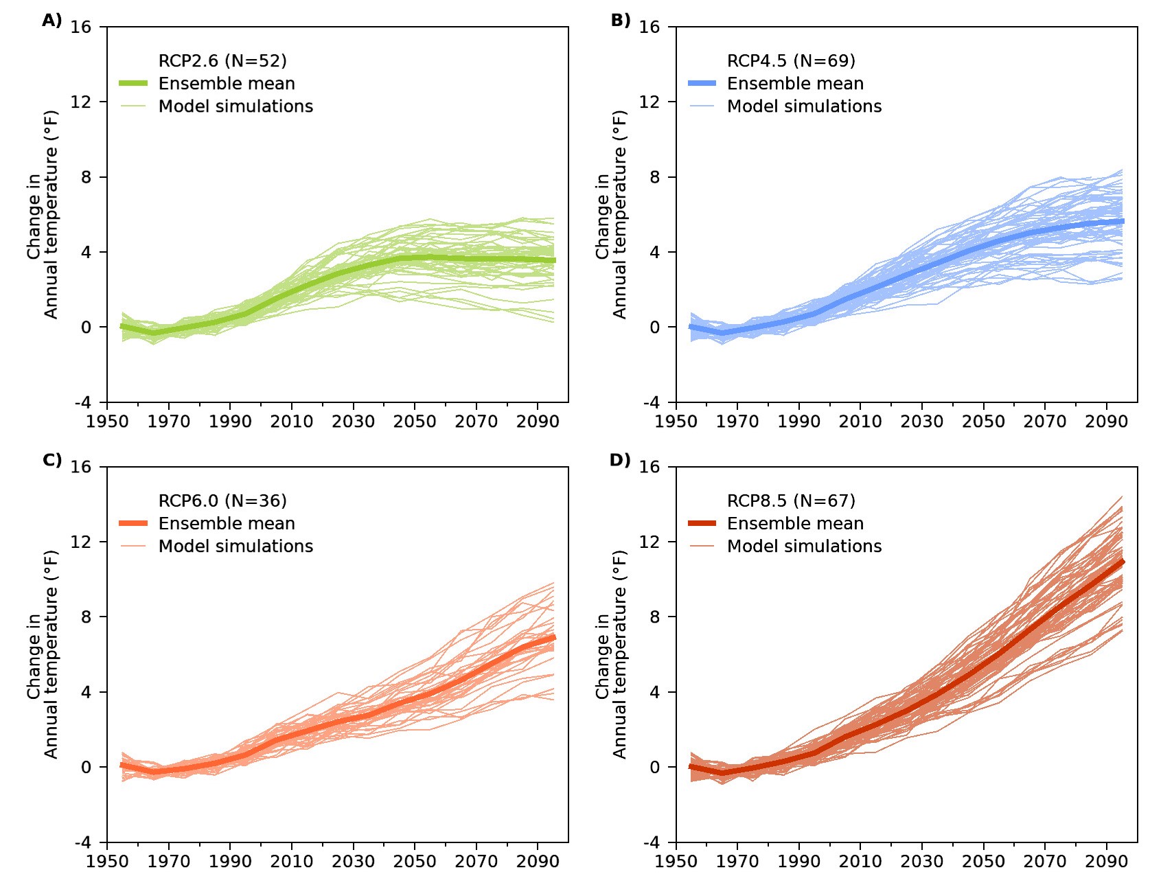
Figure 4-5. Projected change in mean annual air temperature over North America under the four Representative Concentration Pathway (RCP) emission scenarios shown in Figure 4-1. In each plot, the heavy solid line is the 10-year smoothed average of all CMIP5 GCM (fifth Coupled Model Intercomparison Project global climate model) simulations that were run for the RCP, and the lighter lines are the similarly smoothed individual GCM simulations. The total number of simulations conducted for each scenario is indicated by N in the legend. The projections illustrate that, after about 2030, the choice of the RCP becomes the primary controlling factor in projected temperature change and there is increasing spread among the models through time. The plotted data were derived by averaging 1 degree gridded monthly data sets over land in North America between 24.5°N and 53.5°N latitude. Data from the Downscaled CMIP3 and CMIP5 Climate and Hydrology Projections archive at https://gdo-dcp.ucllnl.org/downscaled_cmip_projections/.
Downscaling Climate Projections
Primary methods of downscaling
GCMs depict accurately the main features of the global climate system (Flato et al., 2013; Hayhoe et al. 2019). Even though it is ever improving, spatial resolution can still limit the ability of current GCMs to resolve important details, such as the influence of the diverse topography of the GYA on climate. For regional climate assessments, such as this one, it is desirable to have climate data at a finer spatial scale than is typically produced by GCMs. Several downscaling methods have been developed to derive finer-scale data from GCMs.
The primary downscaling methods are of two types, dynamical and statistical:
-
Dynamical downscaling.—Dynamical methods involve using output from a GCM as input to a separate regional climate model. The regional model also incorporates the physics of atmospheric circulation and surface feedbacks, but at a spatial resolution of tens of kilometers or less over a specific region (e.g., North America). Regional climate models have limitations and require substantial computing power; these constraints limit how many GCM simulations can be practically downscaled using a regional climate model.
-
Statistical downscaling.—Several increasingly complex statistical downscaling methods have emerged since their introduction by Wood et al. (2002). These methods use statistical relationships in observed (i.e., recent) climate data to remove the bias (e.g., differences between modeled and observed temperature) in GCM output and downscale the output to finer spatial resolution. The statistical approach is far less demanding computationally than regional climate models, making it possible to downscale the output from many GCMs.
Statistical downscaling methods also have limitations. For example, the methods are sensitive to the observed data used to establish statistical relationships, and some assume that the relationships will not change in the future, which may be an erroneous assumption. Statistical downscaling is mostly limited to temperature and precipitation; other climate variables are derived from temperature and precipitation by empirical methods. Further information on statistical downscaling and the current leading methods used in the US is provided in Brekke et al. (2013), Bracken (2016), and Pierce et al. (2014).
Downscaling for this Assessment
All downscaling methods transform gridded GCM data onto a finer spatial grid, such as the 4 km by 4 km (2.5 mile by 2.5 mile) grid in this Assessment (Figure 4-6).
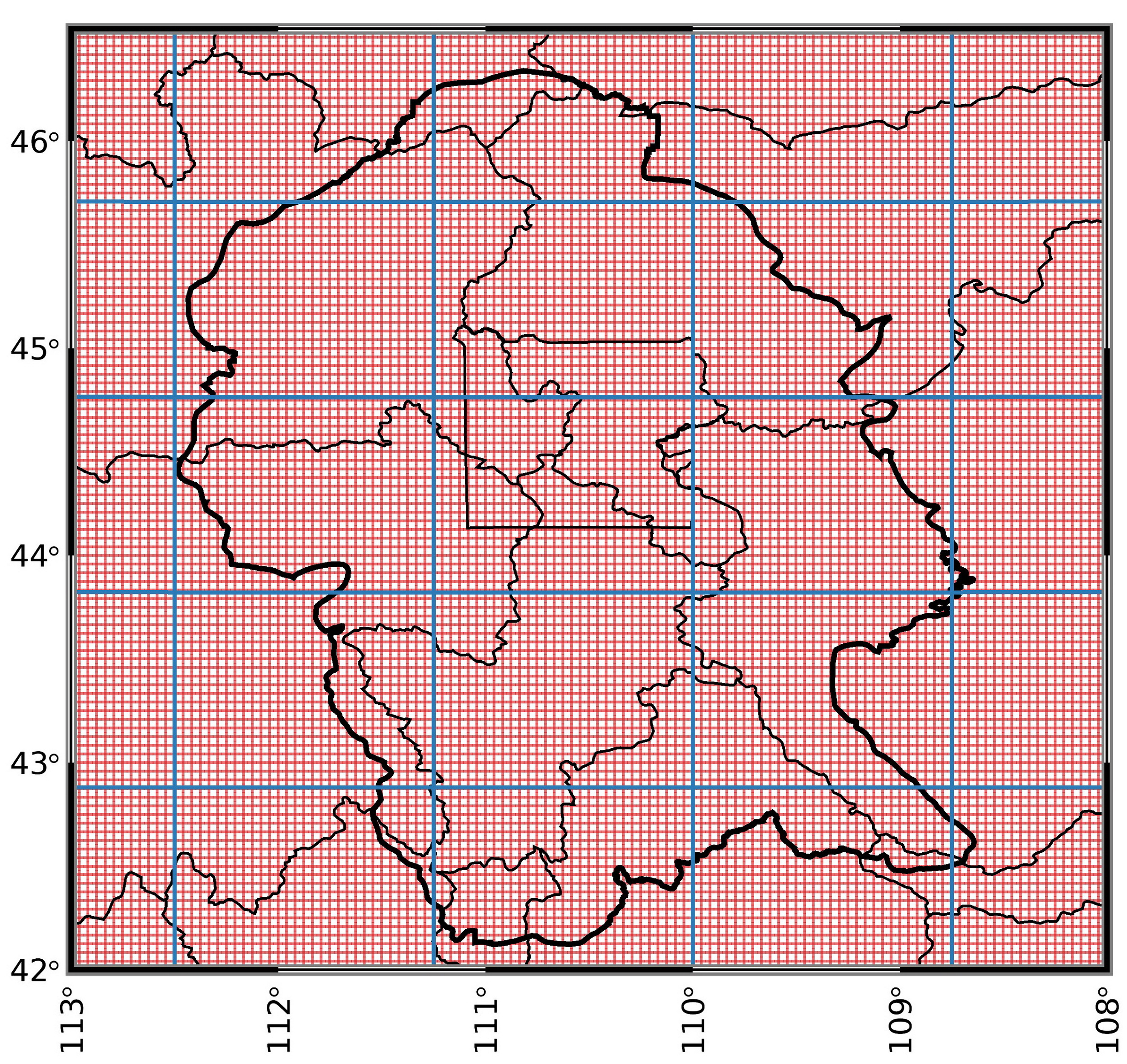
Figure 4-6. Global climate model (GCM) and downscaling grid cells over the Greater Yellowstone Area (GYA). The 0.9° latitude by 1.25° longitude grid cells of the National Center for Atmospheric Research Community Climate System Model (CCSM4) are shown in blue. The CCSM4 is one of the higher spatial resolution GCMs (see Table A4-1 in the appendix to this chapter) in CMIP5 (fifth Coupled Model Intercomparison Project). The red lines indicate the 4-km (2.5 mile) downscaled grid cells used in the Assessment. The full GYA contains 12,960 4-km (2.5-mile) grid cells and there are 800 such grid cells within each GCM cell.
Elevation maps (Figure 4-7) and air temperature maps (Figure 4-8) illustrate how downscaling reveals geographic features that influence the spatial complexity of climate in greater detail than can be resolved by the GCM. It is important to point out, however, that while downscaling often better reflects regional and local topographic features, it is predicated on the accuracy of the original GCM simulations. As such, downscaling cannot reduce issues such as the spread or uncertainty in the simulations, as illustrated in Figures 4-4 and 4-5.
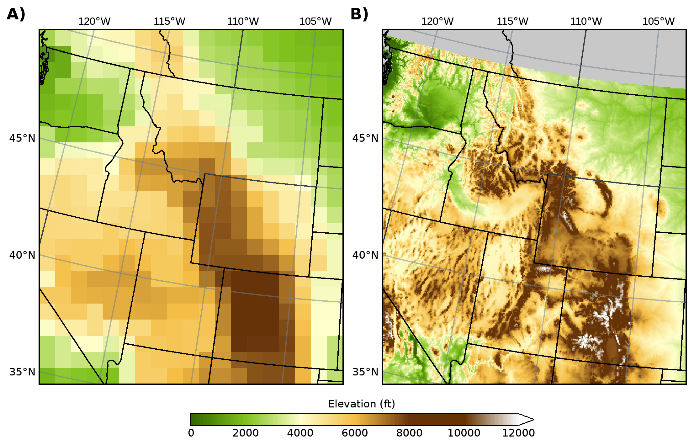
Figure 4-7. Topography of the northern Rocky Mountain region as it is represented on the National Center for Atmospheric Research Community Climate System Model (CCSM4, Table A4-1) (A), and on a 4-km (2.5-mile) grid used in the Assessment (B).
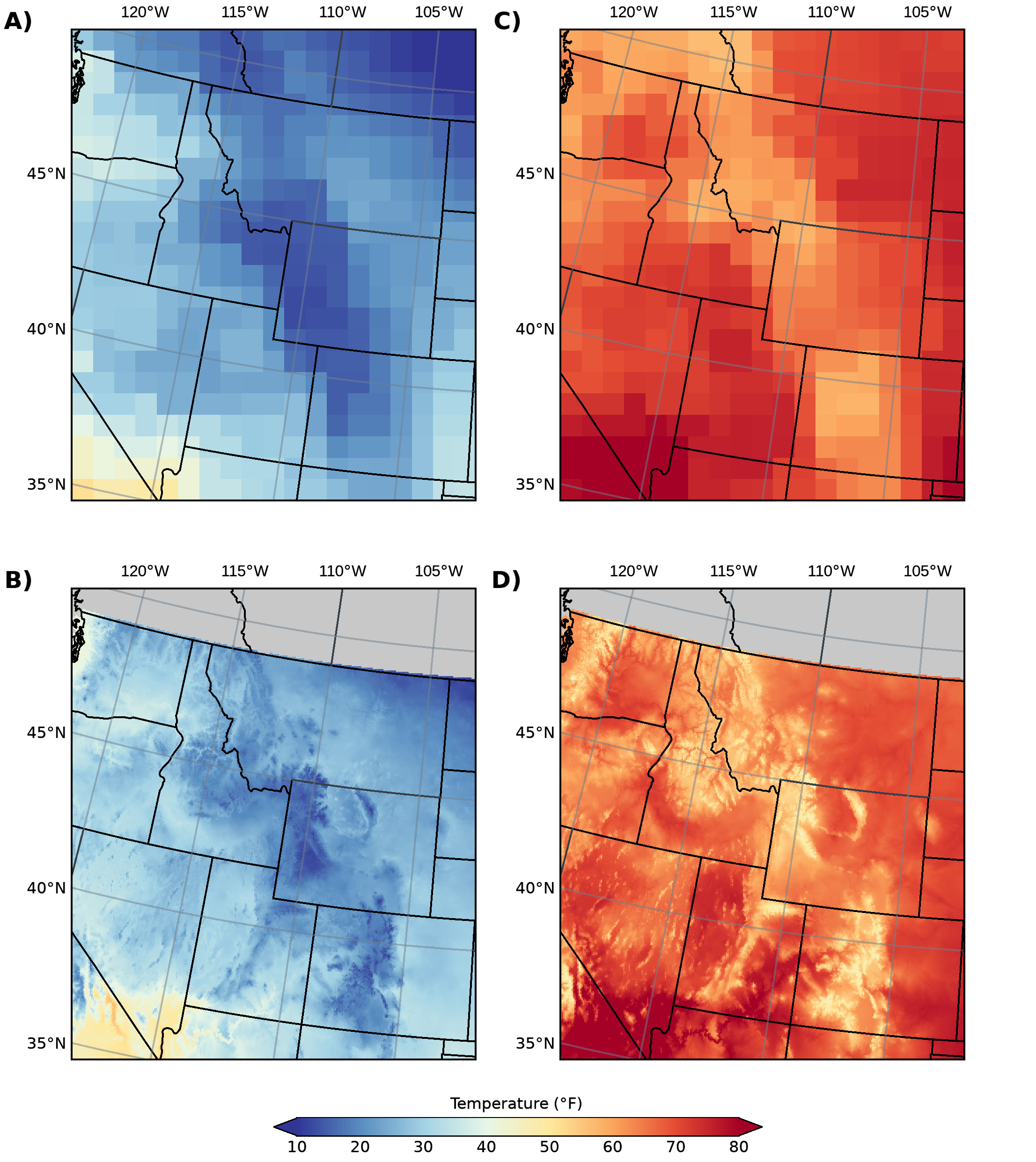
Figure 4-8. Top row: 1980 through 1996 average winter (December through February) air temperature A) and average summer (June through August) air temperature C) as simulated by the National Center for Atmospheric Research Community Climate System Model (CCSM4, Table A4-1). Bottom row: winter B) and summer D) CCSM4 air temperature statistically downscaled to the 4 km by 4 km grid (2.5 mile by 2.5 mile). The downscaled data are from the MACAv2-METDATA data set used in this Assessment.
Climate Projections Used in the Greater Yellowstone Climate Assessment
We based the Assessment on statistically downscaled MACAv2 METDATA climate data (see Table A4-2). The MACAv2-METDATA data set includes 20 CMIP5 GCMs that were statistically downscaled to a 4 km by 4 km (2.5 mile by 2.5 mile) grid using the Multivariate Adaptive Constructed Analogs method (Abatzoglou and Brown 2012; Climatology Lab UC Merced. undated). The modeled data cover the 1950-2005 historical period and the 2006-2099 projection period. The METDATA observational data combines the North American Land Data Assimilation System Phase 2 (Mitchell et al. 2004) and the Parameter-elevation Regressions on Independent Slopes Model (PRISM) (Daly et al. 2008) data to derive gridded data used to bias correct the GCMs (Abatzoglou 2013). The MACAv2-METDATA data were also used in the Montana Climate Assessment (Whitlock et al. 2017). See the appendix to this chapter for further details about the data and data presentations in the Assessment.
In the Assessment, we analyze the two most widely considered 21st-century scenarios (Figure 4-1): RCP4.5 and RCP8.5. We focus on RCP4.5, which is representative of effective mitigation of greenhouse gases by the mid century and include projections for RCP8.5 to cover the full range of possible outcomes. RCP4.5 and RCP8.5 inherently bracket RCP6.0.
An important step is to assess the agreement between observed and modeled temperature and precipitation. Such comparisons evaluate how well the downscaled GCM simulations capture the actual historical period which, assuming they are in good agreement, lends confidence in the 21st-century projections. See the appendix to this chapter for details on the comparison.
Summary
Humans are contributing to global warming through greenhouse gas and aerosol emissions. Climate projections are used to understand, plan for, and mitigate the potential impacts of climate change from present and future emissions.
The process of building projections includes two components: estimating a range of plausible future greenhouse gas and aerosol emissions and incorporating the emissions into global climate models to simulate the response of the Earth system to the scenarios. Projected future emissions are based on assumptions about how energy use, population growth, land-use change, and existing and future technology will affect the emissions. For a given emissions scenario, the climate models collectively produce similar 21st-century temperature trends but with a range in the magnitude of change.
The Assessment uses the two most widely considered 21st-century IPCC scenarios: RCP4.5, which is representative of effective mitigation of greenhouse gases by mid century, and RCP8.5, which is a high-end emissions scenario representative of the unmitigated increase in greenhouse gases. Historical (1950-2005) and future temperature and precipitation data used in the assessment are from 20 CMIP5 global climate models that were downscaled to a 4 km by 4 km (2.5 mile by 2.5 mile) grid over the GYA using the “Multivariate Adaptive Constructed Analogs” (MACA) statistical downscaling method.
Chapter 4 Appendix—A Deeper Look
Tables A4-1 and A4-2 provide a summary of the climate models and climate data used in this report.

Projection uncertainty
Global climate models
Climate projections from global climate models are probabilistic in that they indicate which areas on the Earth have the highest likelihood of climatological change under a given emissions scenario. The output from each model simulation includes internal variability (or weather) as it occurs in the actual climate system, but there is no reason to expect that the simulated weather will match actual observed weather conditions for a particular day or month in the past or in the future. Just as we cannot know which day will be warmest next July, the climate simulations will likely not match future outcomes in detail. They represent the average ways in which future years may differ from present based on a given scenario. Thus, it is the trends and changes in the average climatology that are important in the Assessment, not year-to-year variation (see Chapter 2).
Just as we cannot know which day will be warmest next July, the climate simulations will likely not match future outcomes in detail. They represent the average ways in which future years may differ from present based on a given scenario. Thus, it is the trends and changes in the average climatology that are important in the Assessment, not year-to-year variation (see Chapter 2).
As shown in Figure A4-1, the total uncertainty in the 21st-century climate projections is attributed to three sources: I) the natural variability inherent in the climate system discussed in Chapter 2 (green in Figure A4-1); II) model uncertainty in our knowledge of exactly how much warming GHGs produce in the climate system and how well climate models represent critical processes (the sources of the spread of the individual models shown in Figure 4.5) (blue in Figure A4-1); and III) socioeconomic uncertainty in the societal choices and assumptions used to build emissions scenarios (orange in Figure A4-1) (Hawkins and Sutton 2012; Terando et al. 2020). Over the next 10-20 yr, type I is the largest contributor to total uncertainty. Over the next 30-50 yr, type II emerges as the largest contributor. Much of the type II uncertainty centers around determining the sensitivity of the climate system to a doubling of CO2 in the atmosphere (Sherwood et al. 2020). Over next 60-100 yr, type III dominates total uncertainty.

Figure A4-1. Illustration of the fraction of total uncertainty in decadal average surface air temperature projections for the conterminous United States. The three colors in the graph correspond to the three categories of uncertainty discussed in the text. Figure from Hayhoe et al. (2017) as adopted from Hawkins and Sutton (2009).
GYA climate data
We present the data in various ways: for the entire GYA, the HUC6 watersheds, and selected towns in the GYA. The selected towns represent important population centers and surrounding agriculture areas and they also have available National Weather Service station climate and weather records that we use in our analysis. In our analysis it is also important to note that the level of confidence can decline as the geographic area being considered shrinks (e.g., from the GYA to a town). This is a limitation of downscaling the GCM data over the region. Similarly, some variables (e.g., temperature) exhibit a higher degree of inter-model agreement in the annual average than in the monthly average, particularly early in the 21st century before atmospheric GHG concentrations start to rise substantially.
The projections from the climate models span the period from 1950 to 2099. As discussed in previous chapters, we selected 1986-2005 as our base period for comparison with future periods in the CMIP5 projections. This 20-year period is sufficiently long for computing climatological means; it captures recent observed warming; and allows us to divide the future into four continuous 20-year climatology periods: 2021-2040, 2041-2060, 2061-2080, and 2081-2099. In some figures, we illustrate progressive changes in the 21st-century climate as differences (also referred to as anomalies) obtained by subtracting the 1986-2005 average of a variable from the averages of each future period. We use maps based on Figure 1-3 to highlight spatial variability in the projections. Line graphs and checkerboard plots show the 21st-century changes in monthly averages for each HUC6 watershed and selected towns.
As suggested by Figure 4-5, for a given RCP scenario the 20 GCMs used in this report produce a range of results that varies by climate variable and future year. For example, in 2060 under RCP4.5, all 20 downscaled models project annual warming for the Upper Yellowstone HUC6 watershed, with an all-model mean increase of about 4°F (2.2°C) and range (the difference between the warmest and coldest models) of 6°F (3.3°C) compared to 1950. Thus, the projected temperature increase relative to 1950 is 4 ± 3°F (2.2 ± 1.7°C) or from 1-7°F (0.56-3.9°C). Greater uncertainty exists in projected changes in precipitation than temperature owing to the complexity of representing the underlying processes that result in rain and snow in the GCMs, especially processes related to convection and thunderstorms. Uncertainties in the downscaled MACAv2-METDATA data propagate into the water-balance model simulations.
Comparison of 1950-2018 observed and MACAv2-METDATA temperature and precipitation
The MACAv2-METDATA temperature data are in good agreement with observations (Figure A4-2). The graphs illustrate how temperature decreases with elevation. Less obvious, as indicated by the observations, is that the location of a weather station can strongly influence observed temperature (also precipitation), even over short distances (see Figure 3-1). That influence results from the varied topography of GYA, some of which is not captured at the 4 km (2.5 mile) resolution of the MACAv2-METDATA. An additional factor is that the gridded observational METDATA that is used to bias correct the GCM data is based on interpolation of sparse observations at high elevations.
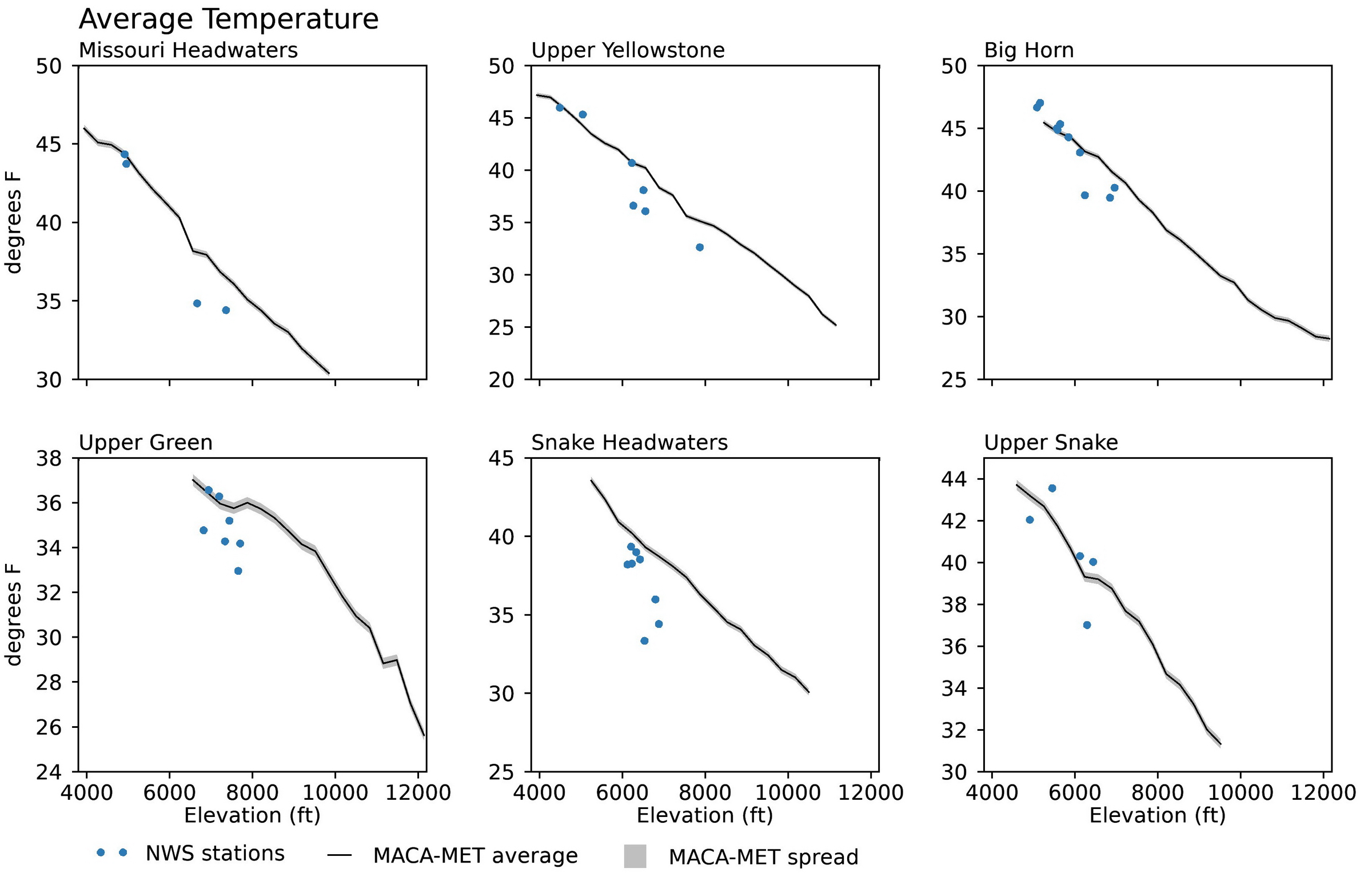
Figure A4-2. Mean annual temperature (y-axis) plotted by elevation (x-axis) for the HUC6 watersheds (Figure 1-3). The solid line is the 1950-2018 20-model mean of the MACAv2-METDATA and the gray bands are the model spread around the mean lines. The blue dots are the mean of the 1950-2018 data from National Weather Service weather stations used in the analysis of historical data in Chapter 3.
The observed and modeled trends in annual air temperature over the HUC6 watersheds are shown in Figure A4-3. The MACAv2-METDATA trend (0.39°F [0.22°C]/decade, significant at the 95% confidence level) is very close to that of the observations (0.35°F [0.19°C]/decade, also significant at the 95% confidence level). Apart from the Big Horn and Snake Headwaters basins, where the trends in the observations are not statistically significant, the HUC6 trends display similar inter-HUC variation and are mostly in agreement with observations.
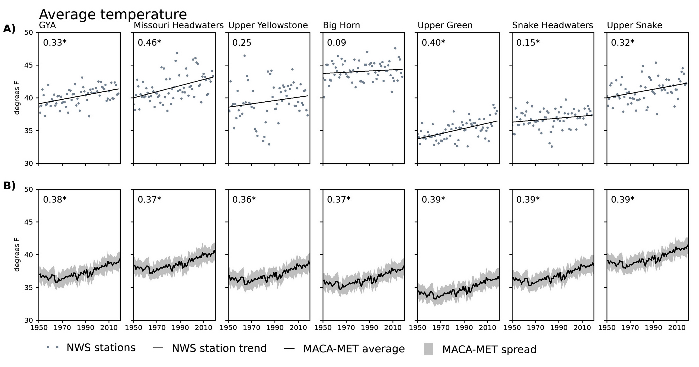
Figure A4-3. Scatter plots of 1950-2018 mean annual temperature for the National Weather Service stations used in Chapter 3 row (A), and time series plots of the MACAv2-METDATA for the Hydrologic Unit Code 6 (HUC6) watersheds row (B). In (A) the gray dots are the observations, and the black lines are linear trend lines fit to the data. In (B), the black lines are the 20-model mean and the gray bands are the model spread around the means. The numbers inset in the upper left of the graphs indicate the trends (in degrees/decade) and an asterisk indicates that the trend is statistically significant at the 95% confidence level.
Overall, the MACAv2-METDATA precipitation data are also in reasonably good agreement with observations (Figure A4-4). The graphs illustrate how, in contrast to temperature, precipitation generally increases with elevation.
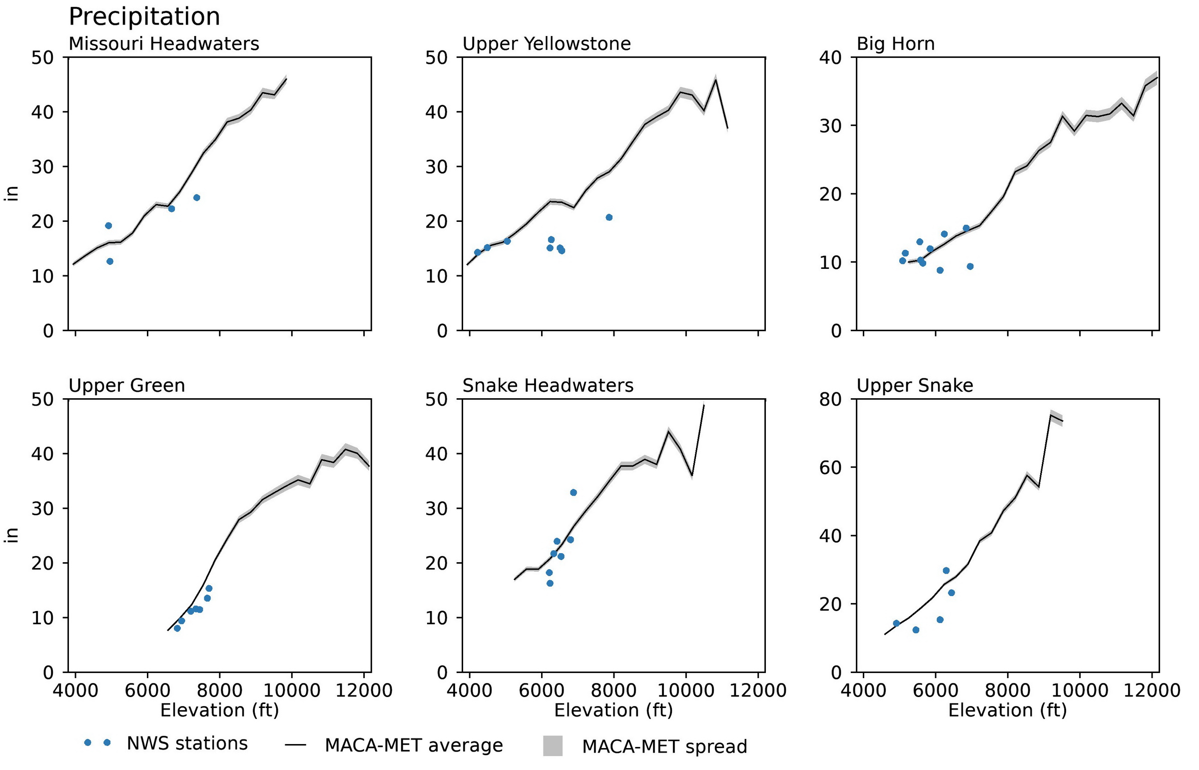
Figure A4-4. Total annual precipitation (y-axis) plotted by elevation (x-axis) for the Hydrologic Unit Code 6 (HUC6) watersheds (Figure 1-3). The solid line is the 1950-2018 20-model average of the MACAv2 METDATA and the gray bands are the model spread around the mean line. The blue dots are the mean of the 1950-2018 data from National Weather Service weather stations used in the analysis of historical data in Chapter 3.
The small, positive trends in precipitation in the MACAv2-METDATA data are all greater than those of the observations (Figure A4-5). Except for the Snake Headwaters watershed, the observed trends are not statistically significant over HUCs or GYA, whereas all the trends in the MACAv2-METDATA are significant. This disagreement in trends is attributed somewhat to differences in the climate models and statistical downscaling, however, as indicated in Figure A4-4. The lack of high elevation observations likely underrepresents total precipitation and is likely a large source of disagreement.
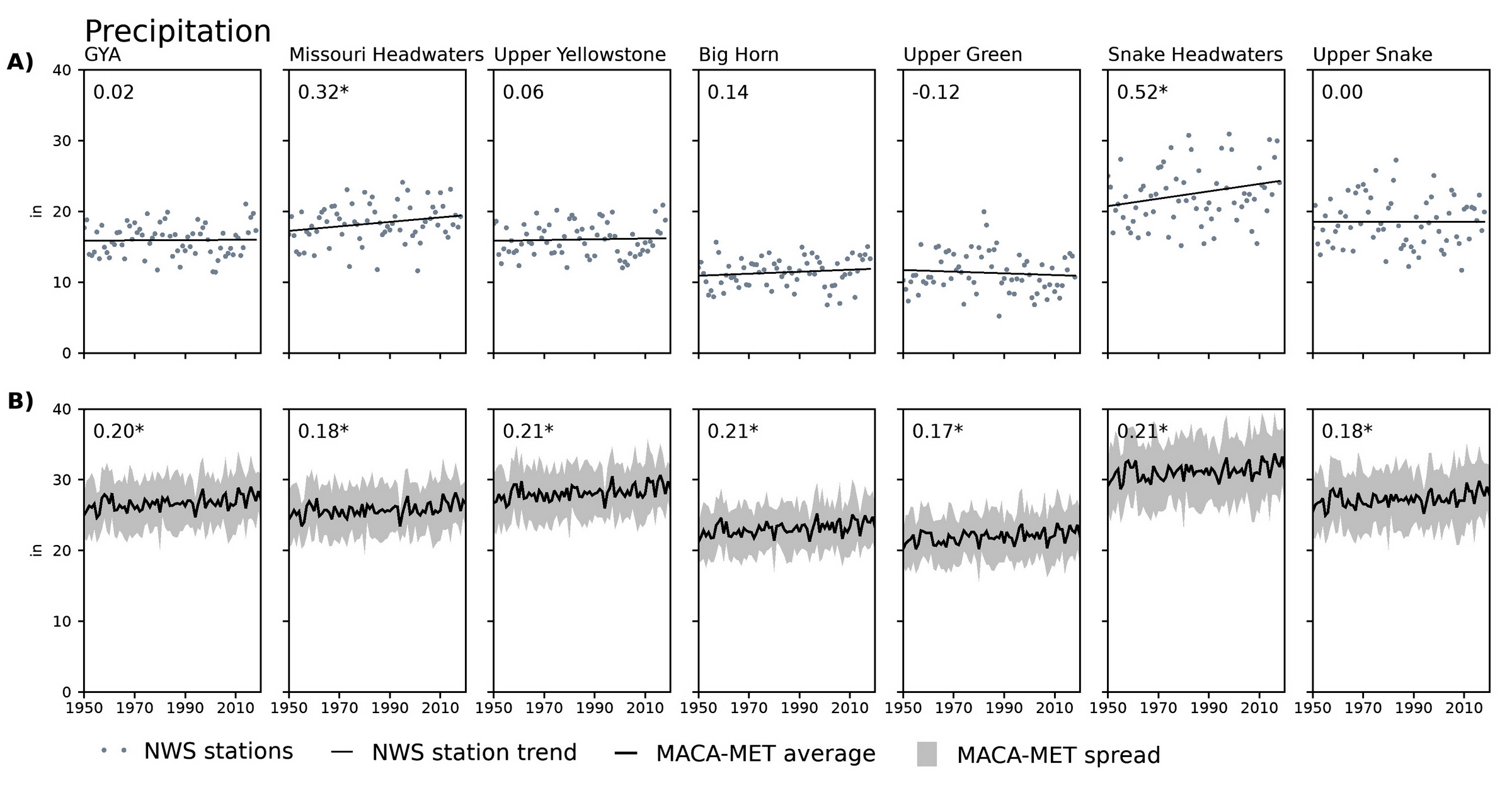
Figure A4-5. Scatter plots of 1950-2018 mean annual precipitation for the National Weather Service stations used in Chapter 3 row (A), and time series plots of the MACAv2-METDATA for the Hydrologic Unit Code 6 (HUC6) basins row (B). In (A) the gray dots are the observations, and the black lines are linear trend lines fit to the data. In (B), the black lines are the 20-model means and the gray bands are the model spread around the means. The numbers inset in the upper left of the graphs indicate the trends (in inches/decade) and an asterisk indicates that the trend is statistically significant at the 95% confidence level.
Literature Cited
Abatzoglou JT. 2013. Development of gridded surface meteorological data for ecological applications and modelling. International Journal of Climatology 33(1):121-31. https://doi.org/10.1002/joc.3413.
Abatzoglou JT, Brown TJ. 2012. A comparison of statistical downscaling methods suited for wildfire applications. International Journal of Climatology 32(5):772-80. https://doi.org/10.1002/joc.2312.
Bracken C. 2016 (Sep). Downscaled CMIP3 and CMIP5 climate projections—addendum [report]. Available online https://gdo dcp.ucllnl.org/downscaled_cmip_projections/techmemo/Downscaled_Climate_Projections_Addendum_Sept2016.pdf. Accessed 30 Sep 2020.
Brekke L, Thrasher BL, Maurer EP, Pruitt T. 2013 (May 7). Downscaled CMIP3 and CMIP5 climate projections: release of downscaled CMIP5 climate projections, comparison with preceding information, and summary of user needs [report]. 104 p. Available online https://gdo-dcp.ucllnl.org/downscaled_cmip_projections/techmemo/downsca…. Accessed 30 Sep 2020.
Clarke L, Edmonds J, Jacoby H, Pitcher H, Reilly J, Richels R. 2007. Scenarios of greenhouse gas emissions and atmospheric concentrations: sub-report 2.1A of synthesis and assessment product 2.1 by the US Climate Change Science Program and the Subcommittee on Global Change Research. Washington DC: Department of Energy, Office of Biological & Environmental Research. 154 p.
Climatology Lab UC Merced. [undated]. MACA [website]. Available online http://www.climatologylab.org. Accessed 30 Sep 2020.
Daly C, Halbleib M, Smith JI, Gibson WP, Doggett MK, Taylor GH, Curtis J, Pasteris PP. 2008. Physiographically sensitive mapping of climatological temperature and precipitation across the conterminous United States. International Journal of Climatology, 28(15):2031-64. https://doi.org/10.1002/joc.1688.
Flato G, Marotzke J, Abiodun B, Braconnot P, Chou SC, Collins W, Cox P, Driouech F, Emori S, Eyring V, Forest C, Gleckler P, Guilyardi E, Jakob C, Kattsov V, Reason C, Rummukainen M. 2013. Evaluation of climate models [chapter 9]. In: Stocker TF, Qin D, Plattner G-K, Tignor M, Allen SK, Boschung J, Nauels A, Xia Y, Bex V, Midgley PM, editors. Climate change 2013: the physical science basis. Contribution of Working Group I to the Fifth Assessment Report of the Intergovernmental Panel on Climate Change. p 741-866. Cambridge UK and New York NY: Cambridge University Press.
Fujino J, Nair R, Kainuma M, Masui T, Matsuoka Y. 2006. Multi-gas mitigation analysis on stabilization scenarios using AIM global model. The Energy Journal 3:343-54.
Hausfather Z, Drake HF, Abbott T, Schmidt GA. 2020. Evaluating the performance of past climate model projections. Geophysical Research Letters 47(1): e2019GL085378. https://doi.org/10.1029/2019GL085378
Hawkins E, Sutton R. 2009. The potential to narrow uncertainty in regional climate predictions. Bulletin of the American Meteorological Society 90:1095-107. https://doi.org/10.1175/2009BAMS2607.1.
Hawkins E, Sutton R. 2012. Time of emergence of climate signals. Geophysical Research Letters 39(1):1-6. https://doi.org/10.1029/2011GL050087.
Hayhoe K, Edmonds J, Kopp RE, LeGrande AN, Sanderson BM, Wehner MF, Wuebbles DJ. 2017. Climate models, scenarios, and projections [chapter 4]. In: Wuebbles DJ, Fahey DW, Hibbard KA, Dokken DJ, Stewart BC, Maycock TK, editors. Climate science special report—fourth national climate assessment, vol I. p 133-160. Washington DC: US Global Change Research Program. https://doi.org/10.7930/J0J964J6.
Hijioka Y, Matsuoka Y, Nishimoto H, Masui M, Kainuma M. 2008. Global GHG emissions scenarios under GHG concentration stabilization targets. Journal of Global Environmental Engineering 13:97-108.
Kellogg WW. 1987. Mankind’s impact on climate—the evolution of an awareness. Climatic Change 10:113-36.
Knutson T, Kossin JP, Mears C, Perlwitz J, Wehner MF. 2017. Detection and attribution of climate change [chapter 4]. In: Wuebbles DJ, Fahey DW, Hibbard KA, Dokken DJ, Stewart BC, Maycock TK, editors. Climate science special report—fourth national climate assessment, vol I. p 114-32. Washington DC: US Global Change Research Program. https://doi.org/10.7930/J0J964J6.
Le Treut H, Somerville R, Cubasch U, Ding Y, Mauritzen C, Mokssit A, Peterson T, Prather M. 2007. Historical Overview of climate change [chapter 1]. In: Solomon S, Qin D, Manning M, Chen Z, Marquis M, Averyt KB, Tignor M, Miller HL, editors. Climate change 2007: the physical science basis. Contribution of Working Group I to the Fourth Assessment Report of the Intergovernmental Panel on Climate Change. p 95-127. Cambridge UK and New York NY: Cambridge University Press.
Mitchell KE, Lohmann D, Houser PR, Wood EF, Schaake JC, Robock A, Cosgrove BA, Sheffield J, Duan Q, Luo L, and others. 2004. The multi-institution North American Land Data Assimilation System (NLDAS): utilizing multiple GCIP products and partners in a continental distributed hydrological modeling system. Journal of Geophysical Research 109 (D7). https://doi.org/10.1029/2003JD003823.
Moss RH, Moss RH, Edmonds JA, Hibbard KA, Manning MR, Rose SK, van Vuuren DP, Carter TR, Emori S, Kainuma M, and others. 2010. The next generation of scenarios for climate change research and assessment. Nature 463:747-56.
National Research Council. 2012. A national strategy for advancing climate modeling. Washington DC: The National Academies Press. 294 p. https://doi.org/10.17226/13430.
[NCAR-UCAR] National Center for Atmospheric Research - University Corporation for Atmospheric Research. [undated]. Climate modeling [webpage]. Available online https://scied.ucar.edu/longcontent/climate-modeling. Accessed 30 Sep 2020.
Pierce DW, Cayan DR, Thrasher BL. 2014. Statistical downscaling using localized constructed analogs (LOCA). Journal of Hydrometeorology 15:2558-85. https://doi.org/10.1175/JHM-D-14-0082.1.
Riahi K, Gruebler A, Nakicenovic N. 2007. Scenarios of long-term socio-economic and environmental development under climate stabilization. Technological Forecasting and Social Change 74(7):887-935.
RCP Database. [undated]. RCP database version 2.05 [website]. Available online https://tntcat.iiasa.ac.at/RcpDb/. Accessed Oct 2020.
Scripps Institute. [undated]. Atmospheric CO2 data: primary Mauna Loa CO2 record [webpage]. Accessible online https://scrippsco2.ucsd.edu/data/atmospheric_co2/primary_mlo_co2_record…. Accessed 29 Mar 2021.
Smith SJ, Wigley TML. 2006. Multi-gas forcing stabilization with the MiniCAM. The Energy Journal 3:373-91.
Taylor KE, Stouffer RJ, Meehl GA. 2012. An overview of CMIP5 and the experiment design. Bulletin of the American Meteorological Society 93:485-98.
Terando A, Reidmiller D, Hostetler SW, Littell JS, Beard Jr TD, Weiskopf SR, Belnap J, Plumlee GS. 2020. Using information from global climate models to inform policymaking—the role of the US Geological Survey. US Geological Survey open-file report 2020-1058. 25 p. https://doi.org/10.3133/ofr20201058
van Vuuren D, den Elzen M, Lucas P, Eickhout B, Strengers B, van Ruijven B, Wonink S, van Houdt R. 2007. Stabilizing greenhouse gas concentrations at low levels: an assessment of reduction strategies and costs. Climatic Change 81:119-59. doi:10.1007/s10584-006-9172-9.
Whitlock C, Cross W, Maxwell B, Silverman N, Wade AA. 2017. 2017 Montana Climate Assessment. Bozeman and Missoula MT: Montana State University and University of Montana, Montana Institute on Ecosystems. 318 p. doi:10.15788/m2ww8w.
Wise MA, Calvin KV, Thomson AM, Clarke LE, Bond-Lamberty B, Sands RD, Smith SJ, Janetos AC, Edmonds JA. 2009. Implications of limiting CO2 concentrations for land use and energy. Science 324:1183-6.
Wood AW, Maurer EP, Kumar A, Lettenmaier DP. 2002. Long-range experimental hydrologic forecasting for the eastern United States. Journal of Geophysical Research-Atmospheres 107(D20):ACL6.1-6.15. https://doi.org/10.1029/2001JD000659.
[1] While the role of GHGs such CO2 in climate warming has been established since the mid-1800s (see the review by Kellogg 1984), the consequences of naturally occurring and human-emitted aerosols are more complex and less well understood. Some aerosols (black carbon or soot) absorb solar radiation and have a warming effect; others are light in color and reflect solar radiation and so have a cooling effect.
[2] The acronym GCM also refers to general circulation models of the atmosphere (AGCM) or oceans (OGCM).
Gallatin River in flood near Big Sky, Montana. Photo courtesy of Scott Bischke.